CS105P SpreadSheet Assignment
Introduction. Larry, one of your coworkers, has been bragging about all the money he is making in the stock market and this has you thinking about your own financial future. As a first step to creating an investment plan you decide to create a budget that shows your income and expenses. Larry also said that, even at a modest rate of return, any investment will grow at an exponential rate and double within 10 years. Larry has a reputation for exaggerating the facts so you decide to also create a worksheet that will test his assertions.
Summary. Create a workbook with two worksheets. Use the figures below as a guide. Use formulas and cell references where appropriate. Use the worksheet "Investment Growth" to calculate the number of years it will take for an initial investment to double at 3%, 6%, and 10 %. Fill in cells F4 and F5 with the correct answer. For example, F6 contains "8 years" because it will take an initial investment of $1,000 about 8 years to double that amount to $2000. (Note, the exact answer is slightly less than 7.5 years but you should round up to the nearest whole number.)
The following is a more detailed description of the assignment.
Workbook
1. Create an Excel workbook with two worksheets (be sure to delete any extra unused worksheets Excel creates for you). Name your worksheets:
![]()
We will first work on the Budget worksheet. First, an image of the completed worksheet will be displayed, then the image will be followed by step-by-step detailed instructions for how to create the worksheet.
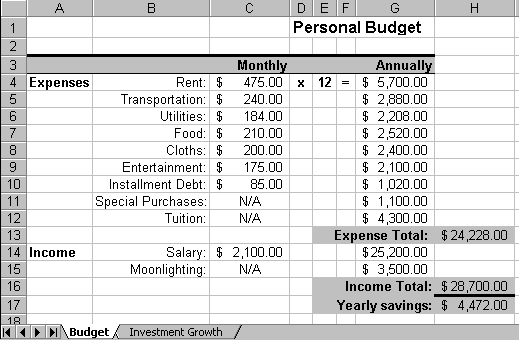
Worksheet 1: Budget
Figure 1.
1. The title "Personal Budget" should have a larger font than the other characters in your worksheet.
2. Row 3 from A-G should be shaded and have a large bold line across the top border.
3. The labels "Monthly" and "Annually" in row 3 are bold and right justified.
4. The label "Expenses" and Income are bold and left justified.
5. The labels in column B should be right justified.
6. The cells with numbers representing dollars should be formatted as Currency.
7. Cells G4:G10 should contain formulas (monthly values * 12). You should type the formula once in cell G4 and then fill down to enter the formula in the remaining cells. (You can do a fill either by doing a copy on the cell, then highlighting the remaining cells, and then pasting. Another way is to highlight the cell, and then "grab" the lower right corner of the cell, with the mouse, then drag the corner down past the remaining cells.)
8. Cells G11 and G12 should contain the numbers given below.
9. Cell H13 should contain the sum() function and contain the sum of cells G4 - G12. (Remember the convention for G4 through G12 is "G4:G12".)
10. Cell H16 should contain the Sum() function and contain the sum of cells G14 and G15. (G14:G15)
11. Cell H17 should contain a formula which is the difference between cells H16 and H13. (H16-H13)
(See Figure 1.)
======================================================================
Next, we will work on the Investment Growth worksheet. First, an image of the completed worksheet will be displayed, then the image will be followed by step-by-step detailed instructions for how to create the worksheet.
Worksheet 2: Investment Growth
Figure 2.
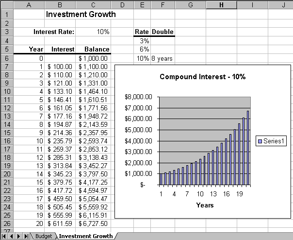
1. The title "Investment Growth" should be underlined and have a larger font than the other characters in your worksheet.
2. The other labels should be bold.
3. The cells A5 - C5 and E3 -F3 should be formatted to have a wide border line along the bottom edge.
4. For the first line in the table of numbers (row 6) enter the values given in the spreadsheet image above.
5. For the second line enter formulas to compute each value. For example,
A7 should have the formula A6+1,
B7 should have the formula C6*$C$3, and
C7 should have the formula C6 + B7.
Note, you will want to use relative and absolute references where appropriate.
6. To get the remaining rows in the table of numbers fill down row 7. (You can do a fill either by doing a copy on the cell, then highlighting the remaining cells, and then pasting. Another way is to highlight the cell, and then "grab" the lower right corner of the cell, with the mouse, then drag the corner down past the remaining cells.)
7. Create a graph showing the growth rate of an investment earning 10% per year. Your graph should look like the graph in Figure 2. (To do the Graph, click on the Graph Icon on the Tool Bar, and use the default bar graph.)
8. Change the value in cell C3 to 3%. Check the table you created in rows 7-26 to see how many years that it takes for the investment to double. Record this amount in cell F4. Repeat for 6% and record this value in cell F5.
9. Change the value in C3 back to 10% so the worksheet you submit looks like the one in Figure 2. (It will look the same except you will have the correct answers in cells F4 and F5.)
(See Figure 2.)